Stochastic Game of Life

We consider a stochastic version of Conway's Game of Life, played on a two-dimensional board. We shall use the following packages,

using Distributions
using StochasticAD
using OffsetArrays
using StaticArrays

Setting up the stochastic Game of Life

Each turn, the standard Game of Life applies the following rules to each cell,

\[\text{dead and 3 neighbours alive} \to \text{ alive}, \\ \text{alive and 0, 1, or 4 neighbours alive} \to \text{ dead}.\]

The cell's status does not change otherwise. In our stochastic version, these rules instead occur with probability 1-θ, while the opposite event has probability θ. To initialize the board at the beginning of the game, we randomly set each cell alive with probability p.

The following high level function sets up the probabilities and provides them to play_game_of_life.

function play(p, θ=0.1, N=12, T=10; log=false)
    # N is the board half-length, T are game time steps
    low = θ
    high = 1-θ
    birth_probs = SA[low, low, low, high, low] # 0, 1, 2, 3, 4 neighbours
    death_probs = SA[high, high, low, low, high] # 0, 1, 2, 3, 4 neighbours
    return play_game_of_life(p, vcat(birth_probs, death_probs), N, T; log)
end

play (generic function with 4 methods)

We can now implement the Game of Life based on the specification. At the end of the game, we return the total number of alive cells.

# A single turn of the game
function update_state(all_probs, N, board_new, board_old)
    for i in -N:N
        for j in -N:N
            neighbours = board_old[i+1, j] + board_old[i-1, j] + board_old[i, j-1] + board_old[i, j+1]
            index = board_new[i,j] * 5 + neighbours + 1
            b = rand(Bernoulli(all_probs[index]))
            board_new[i,j] += (1 - 2 * board_new[i,j]) * b
        end
    end
end

function play_game_of_life(p, all_probs, N, T; log=false)
    dual_type = promote_type(typeof(rand(Bernoulli(p))), typeof.(rand.(Bernoulli.(all_probs)))...) # a hacky way of getting the correct array type
    board = OffsetArray(zeros(dual_type, 2*N + 3, 2*N + 3), -(N+1):(N+1), -(N+1):(N+1)) # center board at (0,0), pad by 1

    # initialize the board
    for i in -N:N
        for j in -N:N
            board[i,j] = rand(Bernoulli(p))
        end
    end
    board_old = similar(board)
    log && (history = [])

    # play the game
    for time_step in 1:T
        copy!(board_old, board)
        update_state(all_probs, N, board, board_old)
        log && push!(history, copy(board))
    end

    if !log
        return sum(board)
    else
        return sum(board), board, history
    end
end

play(0.5, 0.1) # play the game with p = 0.5 and θ = 0.1

99

Differentiating the Game of Life

Let's differentiate the Game of Life!

@show stochastic_triple(play, 0.5) # let's take a look at a single stochastic triple

samples = [derivative_estimate(play, 0.5) for i in 1:10000] # take many samples
derivative = mean(samples)
uncertainty = std(samples) / sqrt(10000)
println("derivative of 𝔼[play(p)] = $derivative ± $uncertainty")

stochastic_triple(play, 0.5) = 60 + 0ε + (4 with probability 282.0ε)
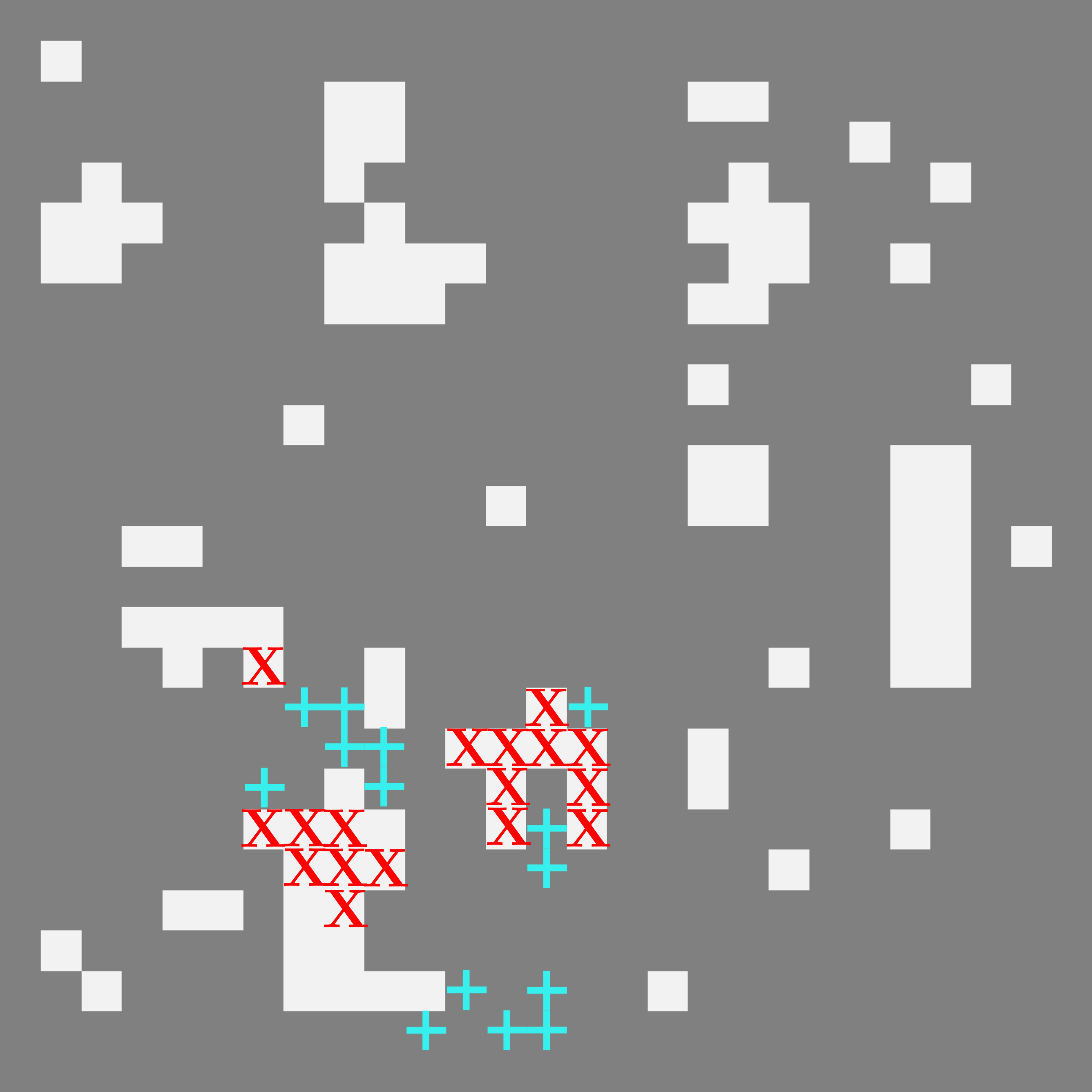
derivative of 𝔼[play(p)] = 163.451 ± 14.688720684642183

The following sketch of the final state of the board for a single run gives some insight into what the stochastic triples are doing. The original board is depicted in grey and white for dead and alive, and the cells which flip from dead to alive in the "alternative" path consider by the triples are marked with + signs, while the cells which flip from alive to dead are marked with X signs.

⠀