Random walk

In this tutorial, we differentiate a random walk over the integers using StochasticAD. We will need the following packages,

using Distributions # defines several supported discrete distributions
using StochasticAD
using StaticArrays # for more efficient small arrays

Setting up the random walk

Let's define a function for simulating the walk.

function simulate_walk(probs, steps, n)
    state = 0
    for i in 1:n
        probs_here = probs(state) # transition probabilities for possible steps
        step_index = rand(Categorical(probs_here)) # which step do we take?
        step = steps[step_index] # get size of step
        state += step
    end
    return state
end

simulate_walk (generic function with 1 method)

Here, steps is a (1-indexed) array of the possible steps we can take. Each of these steps has a certain probability. To make things more interesting, we take in a function probs to produce these probabilities that can depend on the current state of the random walk.

Let's zoom in on the two lines where discrete randomness is involved.

step_index = rand(Categorical(probs_here)) # which step do we take?
step = steps[step_index] # get size of step 

This is a cute pattern for making a discrete choice. First, we sample from a Categorical distribution from Distributions.jl, using the probabilities probs_here at our current position. This gives us an index between 1 and length(steps), which we can use to pick the actual step to take. Stochastic triples propagate through both steps!

Differentiating the random walk

Let's define a toy problem. We consider a random walk with -1 and +1 steps, where the probability of +1 starts off high but decays exponentially with a decay length of p. We take n = 100 steps and set p = 50.

using StochasticAD

const steps = SA[-1, 1] # move left or move right
make_probs(p) = X -> SA[1 - exp(-X / p), exp(-X / p)]

f(p, n) = simulate_walk(make_probs(p), steps, n)
@show f(50, 100) # let's run a single random walk with p = 50
@show stochastic_triple(p -> f(p, 100), 50) # let's see how a single stochastic triple looks like at p = 50

StochasticTriple of Int64:
30 + 0ε + (2 with probability 0.43361358575649517ε)

Time to differentiate! For fun, let's differentiate the square of the output of the random walk.

f_squared(p, n) = f(p, n)^2

samples = [derivative_estimate(p -> f_squared(p, 100), 50) for i in 1:1000] # many samples from derivative program at p = 50
derivative = mean(samples)
uncertainty = std(samples) / sqrt(1000)
println("derivative of 𝔼[f_squared] = $derivative ± $uncertainty")

derivative of 𝔼[f_squared] = 30.15652077676072 ± 0.6974229323126253

Computing variance

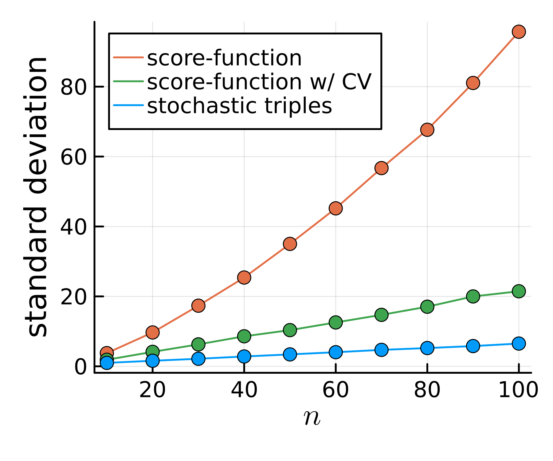
A crucial figure of merit for a derivative estimator is its variance. We compute the standard deviation (square root of the variance) of our estimator over a range of n.

n_range = 10:10:100 # range for testing asymptotic variance behaviour
p_range = 2 .* n_range
nsamples = 10000

stds_triple = Float64[]
for (n, p) in zip(n_range, p_range)
    std_triple = std(derivative_estimate(p -> f_squared(p, n), p)
                     for i in 1:(nsamples))
    push!(stds_triple, std_triple)
end
@show stds_triple

10-element Vector{Float64}:
 0.9856457943667795
 1.5914301525667938
 2.193657290670395
 2.8208789508975722
 3.419976893099299
 4.029648868741822
 4.696535768208758
 5.256497063233989
 5.895326740934028
 6.574072255011413

For comparison with other unbiased estimators, we also compute stds_score and stds_score_baseline for the score function gradient estimator, both without and with a variance-reducing batch-average control variate (CV). (For details, see core.jl and compare_score.jl.) We can now graph the standard deviation of each estimator versus $n$, observing lower variance in the unbiased derivative estimate produced by stochastic triples:

⠀