Differentiable particle filter

Using a bootstrap particle sampler, we can approximate the posterior distributions of the states given noisy and partial observations of the state of a hidden Markov model by a cloud of K weighted particles with weights W.

In this tutorial, we are going to:

implement a differentiable particle filter based on StochasticAD.jl.
visualize the particle filter in $d = 2$ dimensions.
compare the gradient based on the differentiable particle filter to a biased gradient estimator as well as to the gradient of a differentiable Kalman filter.
show how to benchmark primal evaluation, forward- and reverse-mode AD of the particle filter.

Setup

We will make use of several julia packages. For example, we are going to use Distributions and DistributionsAD that implement the reparameterization trick for Gaussian distributions used in the observation and state-transition model, which we specify below. We also import GaussianDistributions.jl to implement the differentiable Kalman filter.

Package dependencies

# activate tutorial project file

# load dependencies
using StochasticAD
using Distributions
using DistributionsAD
using Random
using Statistics
using StatsBase
using LinearAlgebra
using Zygote
using ForwardDiff
using GaussianDistributions
using GaussianDistributions: correct, ⊕
using Measurements
using UnPack
using Plots
using LaTeXStrings
using BenchmarkTools

Particle filter

For convenience, we first introduce the new type StochasticModel with the following fields:

T: total number of time steps.
start: starting distribution for the initial state. For example, in the form of a narrow Gaussian start(θ) = Gaussian(x0, 0.001 * I(d)).
dyn: pointwise differentiable stochastic program in the form of Markov transition densities. For example, dyn(x, θ) = MvNormal(reshape(θ, d, d) * x, Q(θ)), where Q(θ) denotes the covariance matrix.
obs: observation model having a smooth conditional probability density depending on current state x and parameters θ. For example, obs(x, θ) = MvNormal(x, R(θ)), where R(θ) denotes the covariance matrix.

For parameters θ, rand(start(θ)) gives a sample from the prior distribution of the starting distribution. For current state x and parameters θ, xnew = rand(dyn(x, θ)) samples the new state (i.e. dyn gives for each x, θ a distribution-like object). Finally, y = rand(obs(x, θ)) samples an observation.

We can then define the ParticleFilter type that wraps a stochastic model StochM::StochasticModel, a sampling strategy (with arguments p, K, sump=1) and observational data ys. For simplicity, our implementation assumes a observation-likelihood function being available via pdf(obs(x, θ), y).

struct StochasticModel{TType<:Integer,T1,T2,T3}
    T::TType # time steps
    start::T1 # prior
    dyn::T2 # dynamical model
    obs::T3 # observation model
end

struct ParticleFilter{mType<:Integer,MType<:StochasticModel,yType,sType}
    m::mType # number of particles
    StochM::MType # stochastic model
    ys::yType # observations
    sample_strategy::sType # sampling function
end

Kalman filter

We consider a stochastic program that fulfills the assumptions of a Kalman filter. We follow Kalman.jl to implement a differentiable version. Our KalmanFilter type wraps a stochastic model StochM::StochasticModel and observational data ys. It assumes a observation-likelihood function is implemented via llikelihood(yres, S). The Kalman filter contains the following fields:

d: dimension of the state-transition matrix $\Phi$ according to $x = \Phi x + w$ with $w \sim \operatorname{Normal}(0,Q)$.
StochM: Stochastic model of type StochasticModel.
H: linear map from the state space into the observed space according to $y = H x + \nu$ with $\nu \sim \operatorname{Normal}(0,R)$.
R: covariance matrix entering the observation model according to $y = H x + \nu$ with $\nu \sim \operatorname{Normal}(0,R)$.
Q: covariance matrix entering the state-transition model according to $x = \Phi x + w$ with $w \sim \operatorname{Normal}(0,Q)$.
ys: observations.

llikelihood(yres, S) = GaussianDistributions.logpdf(Gaussian(zero(yres), Symmetric(S)), yres)
struct KalmanFilter{dType<:Integer,MType<:StochasticModel,HType,RType,QType,yType}
    # H, R = obs
    # θ, Q = dyn
    d::dType
    StochM::MType # stochastic model
    H::HType # observation model, maps the true state space into the observed space
    R::RType # observation model, covariance matrix
    Q::QType # dynamical model, covariance matrix
    ys::yType # observations
end

To get observations ys from the latent states xs based on the (true, potentially unknown) parameters θ, we simulate a single particle from the forward model returning a vector of observations (no resampling steps).

function simulate_single(StochM::StochasticModel, θ)
    @unpack T, start, dyn, obs = StochM
    x = rand(start(θ))
    y = rand(obs(x, θ))
    xs = [x]
    ys = [y]
    for t in 2:T
        x = rand(dyn(x, θ))
        y = rand(obs(x, θ))
        push!(xs, x)
        push!(ys, y)
    end
    xs, ys
end

simulate_single (generic function with 1 method)

A particle filter becomes efficient if resampling steps are included. Resampling is numerically attractive because particles with small weight are discarded, so computational resources are not wasted on particles with vanishing weight.

Here, let us implement a stratified resampling strategy, see for example Murray (2012), where p denotes the probabilities of K particles with sump = sum(p).

function sample_stratified(p, K, sump=1)
    n = length(p)
    U = rand()
    is = zeros(Int, K)
    i = 1
    cw = p[1]
    for k in 1:K
        t = sump * (k - 1 + U) / K
        while cw < t && i < n
            i += 1
            @inbounds cw += p[i]
        end
        is[k] = i
    end
    return is
end

sample_stratified (generic function with 2 methods)

This sampling strategy can be used within a differentiable resampling step in our particle filter using the use_new_weight function as implemented in StochasticAD.jl. The resample function below returns the states X_new and weights W_new of the resampled particles.

m: number of particles.
X: current particle states.
W: current weight vector of the particles.
ω == sum(W) is an invariant.
sample_strategy: specific resampling strategy to be used. For example, sample_stratified.
use_new_weight=true: Allows one to switch between biased, stop-gradient method and differentiable resampling step.

function resample(m, X, W, ω, sample_strategy, use_new_weight=true)
    js = Zygote.ignore(() -> sample_strategy(W, m, ω))
    X_new = X[js]
    if use_new_weight
        # differentiable resampling
        W_chosen = W[js]
        W_new = map(w -> ω * new_weight(w / ω) / m, W_chosen)
    else
        # stop gradient, biased approach
        W_new = fill(ω / m, m)
    end
    X_new, W_new
end

resample (generic function with 2 methods)

Note that we added a if condition that allows us to switch between the differentiable resampling step and the stop-gradient approach.

We're now equipped with all primitive operations to set up the particle filter, which propagates particles with weights W preserving the invariant ω == sum(W). We never normalize W and, therefore, ω in the code below contains likelihood information. The particle-filter implementation defaults to return particle positions and weights at T if store_path=false and takes the following input arguments:

θ: parameters for the stochastic program (state-transition and observation model).
store_path=false: Option to store the path of the particles, e.g. to visualize/inspect their trajectories.
use_new_weight=true: Option to switch between the stop-gradient and our differentiable resampling step method. Defaults to using differentiable resampling.
s: controls the number of resampling steps according to t > 1 && t < T && (t % s == 0).

function (F::ParticleFilter)(θ; store_path=false, use_new_weight=true, s=1)
    # s controls the number of resampling steps
    @unpack m, StochM, ys, sample_strategy = F
    @unpack T, start, dyn, obs = StochM


    X = [rand(start(θ)) for j in 1:m] # particles
    W = [1 / m for i in 1:m] # weights
    ω = 1 # total weight
    store_path && (Xs = [X])
    for (t, y) in zip(1:T, ys)
        # update weights & likelihood using observations
        wi = map(x -> pdf(obs(x, θ), y), X)
        W = W .* wi
        ω_old = ω
        ω = sum(W)
        # resample particles
        if t > 1 && t < T && (t % s == 0) # && 1 / sum((W / ω) .^ 2) < length(W) ÷ 32
            X, W = resample(m, X, W, ω, sample_strategy, use_new_weight)
        end
        # update particle states
        if t < T
            X = map(x -> rand(dyn(x, θ)), X)
            store_path && Zygote.ignore(() -> push!(Xs, X))
        end
    end
    (store_path ? Xs : X), W
end

Following Kalman.jl, we implement a differentiable Kalman filter to check the ground-truth gradient. Our Kalman filter returns an updated posterior state estimate and the log-likelihood and takes the parameters of the stochastic program as an input.

function (F::KalmanFilter)(θ)
    @unpack d, StochM, H, R, Q = F
    @unpack start = StochM

    x = start(θ)
    Φ = reshape(θ, d, d)

    x, yres, S = GaussianDistributions.correct(x, ys[1] + R, H)
    ll = llikelihood(yres, S)
    xs = Any[x]
    for i in 2:length(ys)
        x = Φ * x ⊕ Q
        x, yres, S = GaussianDistributions.correct(x, ys[i] + R, H)
        ll += llikelihood(yres, S)

        push!(xs, x)
    end
    xs, ll
end

For both filters, it is straightforward to obtain the log-likelihood via:

function log_likelihood(F::ParticleFilter, θ, use_new_weight=true, s=1)
    _, W = F(θ; store_path=false, use_new_weight=use_new_weight, s=s)
    log(sum(W))
end

log_likelihood (generic function with 3 methods)

and

function log_likelihood(F::KalmanFilter, θ)
    _, ll = F(θ)
    ll
end

log_likelihood (generic function with 4 methods)

For convenience, we define functions for

forward-mode AD (and differentiable resampling step) to compute the gradient of the log-likelihood of the particle filter.
reverse-mode AD (and differentiable resampling step) to compute the gradient of the log-likelihood of the particle filter.
forward-mode AD (and stop-gradient method) to compute the gradient of the log-likelihood of the particle filter (without the new_weight function).
forward-mode AD to compute the gradient of the log-likelihood of the Kalman filter.

forw_grad(θ, F::ParticleFilter; s=1) = ForwardDiff.gradient(θ -> log_likelihood(F, θ, true, s), θ)
back_grad(θ, F::ParticleFilter; s=1) = Zygote.gradient(θ -> log_likelihood(F, θ, true, s), θ)[1]
forw_grad_biased(θ, F::ParticleFilter; s=1) = ForwardDiff.gradient(θ -> log_likelihood(F, θ, false, s), θ)
forw_grad_Kalman(θ, F::KalmanFilter) = ForwardDiff.gradient(θ -> log_likelihood(F, θ), θ)

forw_grad_Kalman (generic function with 1 method)

Model

Having set up all core functionalities, we can now define the specific stochastic model.

We consider the following system with a $d$-dimensional latent process,

\[\begin{aligned} x_i &= \Phi x_{i-1} + w_i &\text{ with } w_i \sim \operatorname{Normal}(0,Q),\\ y_i &= x_i + \nu_i &\text{ with } \nu_i \sim \operatorname{Normal}(0,R), \end{aligned}\]

where $\Phi$ is a $d$-dimensional rotation matrix.

seed = 423897

### Define model
# here: n-dimensional rotation matrix
Random.seed!(seed)
T = 20 # time steps
d = 2 # dimension
# generate a rotation matrix
M = randn(d, d)
c = 0.3 # scaling
O = exp(c * (M - transpose(M)) / 2)
@assert det(O) ≈ 1
@assert transpose(O) * O ≈ I(d)
θtrue = vec(O) # true parameter

# observation model
R = 0.01 * collect(I(d))
obs(x, θ) = MvNormal(x, R) # y = H x + ν with ν ~ Normal(0, R)

# dynamical model
Q = 0.02 * collect(I(d))
dyn(x, θ) = MvNormal(reshape(θ, d, d) * x, Q) #  x = Φ*x + w with w ~ Normal(0,Q)

# starting position
x0 = randn(d)
# prior distribution
start(θ) = Gaussian(x0, 0.001 * collect(I(d)))

# put it all together
stochastic_model = StochasticModel(T, start, dyn, obs)

# relevant corresponding Kalman filterng defs
H_Kalman = collect(I(d))
R_Kalman = Gaussian(zeros(Float64, d), R)
# Φ_Kalman = O
Q_Kalman = Gaussian(zeros(Float64, d), Q)
###

### simulate model
Random.seed!(seed)
xs, ys = simulate_single(stochastic_model, θtrue)

([[-0.22612130354931972, -0.7397777673606599], [0.10257548053663229, -0.8756662640277069], [0.30533725356730024, -0.9316721009820819], [0.35223205309819794, -0.5207494524986493], [0.731923949574323, -0.0411758891576422], [0.6201990558051172, 0.4171411401577829], [0.12690539114966093, 0.5693436288027791], [-0.08580438626833706, 0.6147923179674221], [-0.5725463662269625, 0.419836124876971], [-0.7740386185886017, 0.302786999233987], [-0.9261353472714027, 0.07636414522694537], [-1.088941951447555, -0.4309190648605852], [-0.8550506026781588, -0.6854567874131904], [-0.9203484058768842, -1.0901910821078156], [-0.41552856810697797, -1.4245984007439212], [0.21103726131037975, -1.5082912964261341], [0.724399532207084, -1.166642874879663], [1.4186299786585466, -0.6757136319755501], [1.5333776723943078, -0.05733606912093908], [1.5666966620481166, 0.6465869841340743]], [[-0.3335699301254105, -0.6822297518733397], [0.10649860667465556, -0.9699927550775741], [0.0722098332304546, -0.8941779163980673], [0.5323611415822864, -0.4705535197109296], [0.8620176235034201, -0.07448895682829396], [0.6833355853473924, 0.43030537701154553], [0.18492848687873895, 0.37787869451568495], [-0.07727788092087334, 0.878333405938457], [-0.7381646694408511, 0.3697701331751778], [-0.8385889725531148, 0.31656170522011723], [-0.8713259022393924, 0.14513285008552113], [-1.089904609366039, -0.3867653341275366], [-0.866108973417278, -0.7565340096273592], [-0.8898141908866023, -1.2102559728450681], [-0.39331068259567104, -1.4244448023403207], [0.1617976246325039, -1.4410648754368118], [0.6568484699164703, -1.2687269457761559], [1.347749035820413, -0.5475977604805508], [1.4864602942860088, -0.08613761533171067], [1.3693546099408112, 0.6275404072590013]])

Visualization

Using particle_filter(θ; store_path=true) and kalman_filter(θ), it is straightforward to visualize both filters for our observed data.

m = 1000
kalman_filter = KalmanFilter(d, stochastic_model, H_Kalman, R_Kalman, Q_Kalman, ys)
particle_filter = ParticleFilter(m, stochastic_model, ys, sample_stratified)

Main.ParticleFilter{Int64, Main.StochasticModel{Int64, typeof(Main.start), typeof(Main.dyn), typeof(Main.obs)}, Vector{Vector{Float64}}, typeof(Main.sample_stratified)}(1000, Main.StochasticModel{Int64, typeof(Main.start), typeof(Main.dyn), typeof(Main.obs)}(20, Main.start, Main.dyn, Main.obs), [[-0.3335699301254105, -0.6822297518733397], [0.10649860667465556, -0.9699927550775741], [0.0722098332304546, -0.8941779163980673], [0.5323611415822864, -0.4705535197109296], [0.8620176235034201, -0.07448895682829396], [0.6833355853473924, 0.43030537701154553], [0.18492848687873895, 0.37787869451568495], [-0.07727788092087334, 0.878333405938457], [-0.7381646694408511, 0.3697701331751778], [-0.8385889725531148, 0.31656170522011723], [-0.8713259022393924, 0.14513285008552113], [-1.089904609366039, -0.3867653341275366], [-0.866108973417278, -0.7565340096273592], [-0.8898141908866023, -1.2102559728450681], [-0.39331068259567104, -1.4244448023403207], [0.1617976246325039, -1.4410648754368118], [0.6568484699164703, -1.2687269457761559], [1.347749035820413, -0.5475977604805508], [1.4864602942860088, -0.08613761533171067], [1.3693546099408112, 0.6275404072590013]], Main.sample_stratified)

### run and visualize filters
Xs, W = particle_filter(θtrue; store_path=true)
fig = plot(getindex.(xs, 1), getindex.(xs, 2), legend=false, xlabel=L"x_1", ylabel=L"x_2") # x1 and x2 are bad names..conflicting notation
scatter!(fig, getindex.(ys, 1), getindex.(ys, 2))
for i in 1:min(m, 100) # note that Xs has obs noise.
    local xs = [Xs[t][i] for t in 1:T]
    scatter!(fig, getindex.(xs, 1), getindex.(xs, 2), marker_z=1:T, color=:cool, alpha=0.1) # color to indicate time step
end

xs_Kalman, ll_Kalman = kalman_filter(θtrue)
plot!(getindex.(mean.(xs_Kalman), 1), getindex.(mean.(xs_Kalman), 2), legend=false, color="red")

"pf_1.png"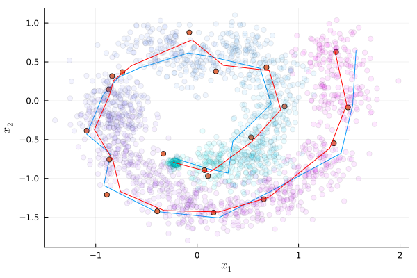

Bias

We can also investigate the distribution of the gradients from the particle filter with and without differentiable resampling step, as compared to the gradient computed by differentiating the Kalman filter.

### compute gradients
Random.seed!(seed)
X = [forw_grad(θtrue, particle_filter) for i in 1:200] # gradient of the particle filter *with* differentiation of the resampling step
Random.seed!(seed)
Xbiased = [forw_grad_biased(θtrue, particle_filter) for i in 1:200] # Gradient of the particle filter *without* differentiation of the resampling step
# pick an arbitrary coordinate
index = 1 # take derivative with respect to first parameter (2-dimensional example has a rotation matrix with four parameters in total)
# plot histograms for the sampled derivative values
fig = plot(normalize(fit(Histogram, getindex.(X, index), nbins=20), mode=:pdf), legend=false) # ours
plot!(normalize(fit(Histogram, getindex.(Xbiased, index), nbins=20), mode=:pdf)) # biased
vline!([mean(X)[index]], color=1)
vline!([mean(Xbiased)[index]], color=2)
# add derivative of differentiable Kalman filter as a comparison
XK = forw_grad_Kalman(θtrue, kalman_filter)
vline!([XK[index]], color="black")

"pf_2.png"

The estimator using the new_weight function agrees with the gradient value from the Kalman filter and the particle filter AD scheme developed by Ścibior and Wood, unlike biased estimators that neglect the contribution of the derivative from the resampling step. However, the biased estimator displays a smaller variance.

Benchmark

Finally, we can use BenchmarkTools.jl to benchmark the run times of the primal pass with respect to forward-mode and reverse-mode AD of the particle filter. As expected, forward-mode AD outperforms reverse-mode AD for the small number of parameters considered here.

# secs for how long the benchmark should run, see https://juliaci.github.io/BenchmarkTools.jl/stable/
secs = 1

suite = BenchmarkGroup()
suite["scaling"] = BenchmarkGroup(["grads"])

suite["scaling"]["primal"] = @benchmarkable log_likelihood(particle_filter, θtrue)
suite["scaling"]["forward"] = @benchmarkable forw_grad(θtrue, particle_filter)
suite["scaling"]["backward"] = @benchmarkable back_grad(θtrue, particle_filter)

tune!(suite)
results = run(suite, verbose=true, seconds=secs)

t1 = measurement(mean(results["scaling"]["primal"].times), std(results["scaling"]["primal"].times) / sqrt(length(results["scaling"]["primal"].times)))
t2 = measurement(mean(results["scaling"]["forward"].times), std(results["scaling"]["forward"].times) / sqrt(length(results["scaling"]["forward"].times)))
t3 = measurement(mean(results["scaling"]["backward"].times), std(results["scaling"]["backward"].times) / sqrt(length(results["scaling"]["backward"].times)))
@show t1 t2 t3

ts = (t1, t2, t3) ./ 10^6 # ms
@show ts

(30.16 ± 0.68, 43.1 ± 1.8, 1715.648436 ± NaN)